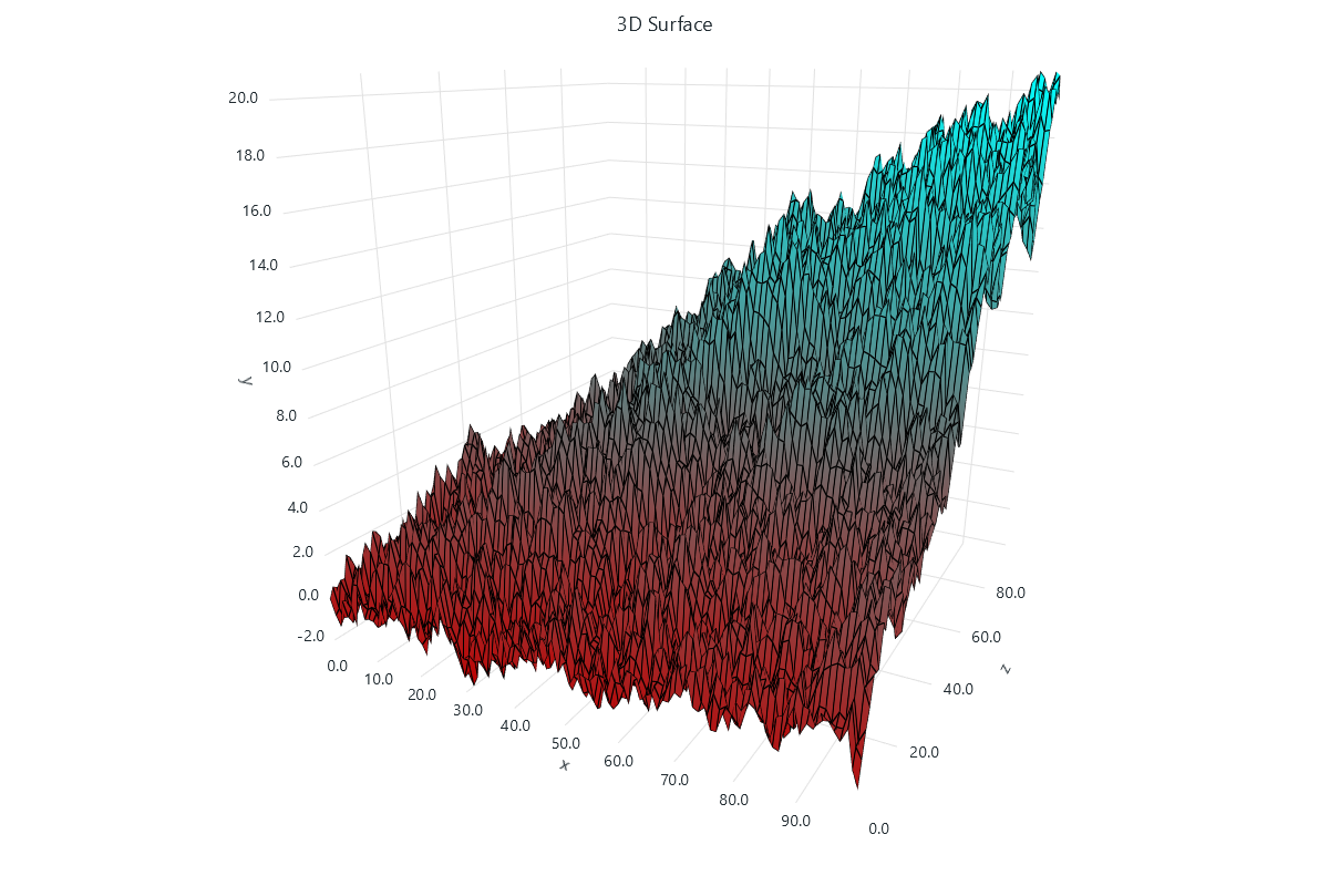
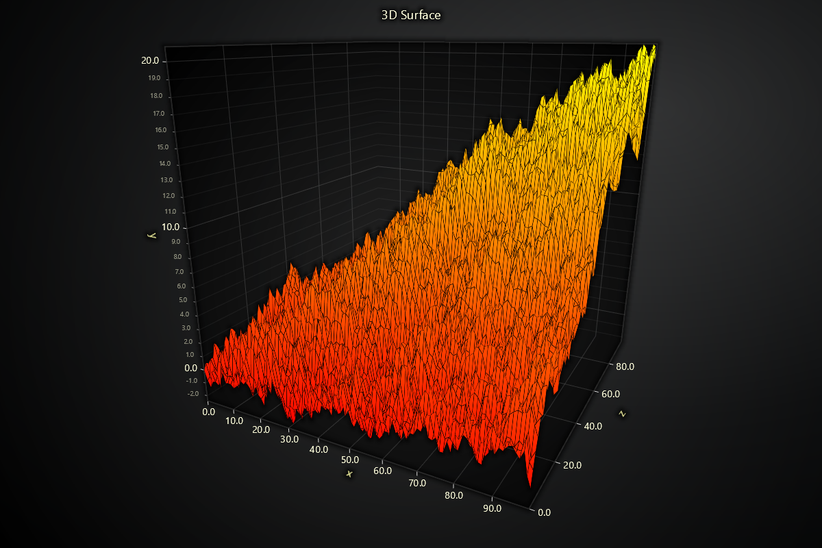
3D Surface
3D surfaces can be created using Chart3D and Surface Grid Series. This series is optimized for massive amounts of surface grid data.
The grid is defined by imagining a plane along X and Z axis, split to < COLUMNS > (cells along X axis) and < ROWS > (cells along Z axis). The total amount of < CELLS > in a surface grid is calculated as columns * rows. Each < CELL > can be associated with DATA from a user data set.
See also Scrolling 3D Surface.
Creating 3D Surface
series = chart.add_surface_grid_series(columns=3, rows=3)
Configuring 3D Surface Coordinates
These methods allow you to define the spatial positioning of 3D Surface samples.
Set Start Coordinate
# Set the start coordinate to (0, 0)
series.set_start(x=0, z=0)
Set End Coordinate
# Set the end coordinate to (100, 50)
series.set_end(x=100, z=50)
Set Step Between Samples
# Set the step between samples to 10 in X and 5 in Z
series.set_step(x=10, z=5)
Data input and Intensity Invalidation
Invalidate Intensity Values
This method helps update the 3D Surface's intensity values:
# Define a 2D matrix for new intensity values:
data_matrix = [
    [1.0, 2.0, 3.0],
    [2.5, 3.5, 4.0],
    [3.0, 4.0, 5.0]
]
# Update the intensity values.
series.invalidate_intensity_values(data=data_matrix)
Intensity interpolation
# Enable smooth intensity interpolation:
series.set_intensity_interpolation(True)
Invalidate Height Map
Similar to intensity invalidation, you can update the surface's vertical (Y-axis) heights in a sub-region:
# Define a matrix of new height values
height_matrix = [
    [0.5, 1.0, 0.8],
    [0.7, 1.2, 0.9],
    [0.6, 1.1, 1.3],
]

# Update starting at column 0, row 0
series.invalidate_height_map(data=height_matrix, column_index=0, row_index=0)
invalidate_height_map(data, column_index, row_index)Replaces the height values (Y) for the grid cells beginning at the given column/row.
Contour Lines
Add contour lines to visualize specific value thresholds on 3D surfaces.
Basic Contours
series.set_contours(
    levels=[
        {'value': 10},
        {'value': 50},
        {'value': 90}
    ]
)
Styled Contours
series.set_contours(
    levels=[
        {
            'value': 25,
            'stroke_style': {'thickness': 2, 'color': '#0000FF'}
        },
        {
            'value': 75,
            'stroke_style': {'thickness': 3, 'color': '#FF0000'}
        }
    ]
)
Extrapolating surface data from scatter data set
One common way of using surface charts is to extrapolate a surface height map from a scattered 3D data set. For example, see the video below, which displays both Raw samples (as scatter points) and the extrapolated surface:
Culling, Depth Test & Shading
Control back-face/front-face culling, depth buffering, and shading style on the 3D surface:
# Disable culling to render both sides of surface polygons
series.set_cull_mode('disabled')       # options: 'disabled', 'cull-back', 'cull-front'

# Turn off depth testing so overlapping parts draw in append order
series.set_depth_test_enabled(False)

# Choose between Phong (smooth) or simple flat shading
series.set_color_shading_style(
    phong_shading=True,                # True = Phong, False = flat
    specular_reflection=0.5,           # specular strength [0–1]
    specular_color='#FFFFFF'           # highlight color
)
-
set_cull_mode(mode)Controls which polygon faces to discard:"cull-back"(default) discards faces pointing away from camera"cull-front"discards faces pointing toward camera"disabled"renders both sides
-
set_depth_test_enabled(enabled)Enables/disables GPU depth buffering (occlusion) for this mesh. -
set_color_shading_style(phong_shading, specular_reflection, specular_color)Switches between realistic Phong shading and a simple lighting model, with tunable specular highlight.
Customizing Fill Coloring
Set Palette Coloring
import lightningchart as lc
# Create a palette that transitions from blue to red:

series.set_palette_coloring(
  steps=
[
    {'value': 0, 'color': ('#0000FF')},
    {'value': 50, 'color': ('red')}
]
, look_up_property='value'
, interpolate=True
)

# With formatted legend display:
series.set_palette_coloring(
    steps=[
        {'value': 0, 'color': '#0000FF'},
        {'value': 100, 'color': '#FF0000'},
    ],
    look_up_property='value',
    formatter_precision=2,           # Decimal places
    formatter_unit='mag',             # Unit suffix
    formatter_scale=1.5,              # Scale values
    formatter_type='scientific',      # 'standard', 'compact', 'engineering', 'scientific'
    formatter_operation='floor',      # 'none', 'round', 'ceil', 'floor'
)
Solid Fill Color
import lightningchart as lc

# Set the fill color to a light gray:
series.set_color((200, 200, 200))
Removing Color
# Remove the fill color:
series.set_empty_color_fill()
Wireframe Configuration
Set Wireframe Stroke
import lightningchart as lc

# Set a wireframe with 2px thickness in black:
series.set_wireframe_stroke(thickness=2, color='black')
Hide Wireframe
# Hide the 3D surface wireframe:
series.hide_wireframe()
Series Utility Methods:
# Set a name for the series (used in legend and tooltip)
series.set_name("3D Surface")

# Highlight the series fully (1.0 = max highlight)
series.set_highlight(1.0)

# Enable or disable theme-based visual effects
series.set_effect(True)

# Toggle series visibility (False hides it from view)
series.set_visible(True)

# Permanently remove the series from the chart
series.dispose()
Legend
Please see common legend section.